Impact of Resources and Technology on Farming Production in Northwestern China

1           Introduction

The rapid growth in China’s farming production from 1979 has been outstanding by international standards. The success of the rural reform has attracted extensive interest in studying the effects of farming inputs on Chinese farming production. A representative selection of studies includes Wiens (1982), Lin (1992), Wen (1993), Xu (1999), and Carter et al. (1999). Use of the general production function is the primary approach, which estimates the marginal productivity and output elasticity of the main production factors (Lin, 1992; Wiemer, 1994). To estimate farming production, a common approach in these studies is to classify farming inputs into different categories including land, labor, and material inputs (fertilizer, machinery, pesticide, herbicide, seed, and so on). It is generally accepted that the rapid growth of farming production in China was due to the increasing technological and industrial inputs that steamed from economic reforms in the 1970s and 1980s. Besides these common regulators, water resource is also a key factor in the agricultural development in northwestern China, where the arid climate limits large scale intensive farming (Huang and Rozelle, 1995 and 1997, CASS, 2000). With much wasteland, light, and heat resources but very limited precipitation, the modern agriculture in this area has been largely dependent on irrigation (Tao and Wei, 1996; Wen and Pimentel, 1998).

Focusing on the effects of water utilization on farming production, this paper presents a comprehensive analysis on the impact of resources, irrigation in particular, and technology on the farming production in northwestern China. By applying the Cobb‑Douglas model to historical data in the region, this study aimed to identify and evaluate the relationship between farming output and specified inputs in resources and technology. Contributions of farming inputs on output were also quantified, by decomposing the growth of farming production as sum of the contributions by individual inputs. By characterizing on the spatial variations of water utilization and technological inputs in farming, the results of this study shed new light to the nature of farming production in this arid region of northwestern China, and are anticipated to be useful in optimizing the agricultural structure of the region for a sustainable development.

2           Materials and methods

2.1         Brief description of the region

The northwestern region of China consists of five provincial districts, i.e., Shaanxi province, Ningxia Hui Autonomous Region, Gansu province, Qinghai province, and Xinjiang Uygur Autonomous Region (Figure 1). The total area of the region is 3.09 million km², comprising approximately one-third of China’s land area. Arid regions occupy a vast area in northwestern China, where the mean annual rainfall is less than 250 mm. Within the region, annual precipitation in the western plains is only in the range of 50 to 150 mm, and less than 25 mm in the Taklimakan Desert. The annual evaporation, however, is more than 1,400 mm in average, and about 2,000 to 3,000 mm in the desert areas.

The total amount of water resources is 487.4 billion m³ in this region, accounting for only 13.7% of the national total amount.  The limited water resources are concentrated within Qinghai and Xinjiang.  Because of the arid climate, only a small portion of the total area in the region is used for farming production (about 0.13 million km²). Irrigated farmlands are primarily located in Ningxia Plain, Hexi Corridor Region in Gansu and the northern oasis area of Xinjiang. In other parts of this region, most of the sown area is rain-fed, with scattered irrigated areas. Except for Xinjing, the farmland productivity and labor productivity in the region are lower than the national average (CASS, 2000).

2.2         Variables and data

In this study, we used annual gross value of farming production (P, RMB) for the estimation of farming output. The production values for different years had been deflated/inflated to the constant price of 1978 to make meaningful comparisons over time. To examine the effects of resources utilization and technology application, we chose irrigation ratio (I, dimensionless), farming labor (L, person), fertilizer application (F, ton), and farm machinery (M, kW ha^-1) as input variables. The irrigation ratio was defined as the decimal fraction of irrigated area to the total sown area in each provincial district. Preliminary data analysis indicated that the sown area in the region did not change much during the study period. Therefore, the irrigation ratio was an important factor in representing the input of water resources in the farming activities. Because the effect of the changes in non-irrigated (rainfed) farmland was insignificant due to the very low farming efficiency (Rathore, 1996), the farming output in rainfed land was roughly assumed constant in the production model. The data on workers actually engaged in farming was unavailable. Therefore, we used the workers in agricultural activities (animal husbandry, sideline activities, fisheries, forestry, and water conservancy) for the farming labor. The technological inputs were represented by the use of chemical fertilizer and farming machinery, which reflected the industrial inputs in the region that has a major impact on farm production (Cater et al., 1999, Mead, 2000)

The above output and input variables were defined over the whole northwestern region, and also for each provincial district, i.e., Shaanxi, Gansu, Ningxia, Qinghai and Xinjiang. Data for all the above variables were obtained from the official publications of the Chinese government (China DCSNBS, 1999; China AEC, 1999) for 21 years, from 1978 through 1998.

2.3         Descriptive statistics

Descriptive statistics of the data were preformed firstly to characterize the temporal trends and spatial variations of framing output and input variables in the five provincial districts during 1978-1998. In addition to the overall rate of change, the trend analysis also provided detailed information on the dynamic fluctuations of the variables. Correlation analysis was employed to examine the associations of the farming output with the selected inputs, and among the inputs themselves. Correlation analysis in this study was based on the Pearson correlation model, which reflects the degree of linear relationship between any two variables.

2.4         Modeling with the Cobb-Douglas function

The Cobb-Douglas production function empirically describes the relationship between output and specified inputs, and quantifies the effects of pertinent inputs such as irrigation, labor, and technology on the output (Fan, 1991; Lin, 1992; Ahmad et al., 1995; Kaufmann and Snell, 1997; Carter and Zhang, 1998; Lindert, 1999). Comparing to other approaches (such as DEA Malmquist Index), the Cobb-Douglas model has the merits in consistency with economic theory, flexibility in data transformation, and less sensitivity to extreme observation error or background noise in the data (Sharma et al., 1997). Therefore, we choose the Cobb-Douglas model to characterize the impact of resources and technological factors on the farming production in northwestern China, by fitting our data into the following function:

(1)

where the α’s are the model parameters to be estimated. The parameter α₀ represents the model bias including the error caused by missing some of the important region-specific input variables in the formulation.  The parameters α₁ through α₄ reflect the shares of the corresponding input variables to output.  Because the size of the districts varies greatly, to prevent the heteroscedastic problem, the output as well as the input variables were normalized by the values in each provincial district in 1978, the first year of our dataset. Thus, all the variables in 1978 were fixed at unity, and the normalized data represented the relative values to the corresponding 1978 level. To estimate the model parameters, we transformed the equation into logarithmic form,

(2)

Ridge regression was performed to estimate the parameters in the Cobb-Douglas model (Eq. 2) since some input variables were inter-correlated. When multicolinearity occurs, the variances are large and far from the true value. By imposing some bias on the regression coefficients and shrinking their variance, ridge regression could result in more stable equations with highly multicollinear data, and thus requires less data than typically needed by least squares methods (Morris, 1982, Pagel and Lunebery, 1985, Orr, 1996).

A preliminary check on the skewness and kurtosis of the data indicated that most of the data series showed strongly positive skewness. The departures from normality were also obvious from the inspection on the difference between expected frequencies of a normal distribution and the obtained frequencies in the data histograms. Therefore, it was also statistically appropriate to transform the variables into the logarithmic forms shown in Eq. (2).

2.5         Contributions of inputs to output

Theoretically, the Cobb-Douglas production function assumes a linear relationship between the growths of output and inputs. This linear relationship can be expressed as the following by introducing a residual term to close the equation (Mead, 2000, Fedderke, 2001, Xu, 1999),

(3)

where the residual changes in output, ε, is normally termed as total factor productivity, and the α’s are the output elasticities with respect to the input variables, evaluated by regression analysis on the Cobb-Douglas production function (Eq. 2). The regression constant α₀ was not included in Eq. (3) since this linear relationship accounted for only the growth of variables with time. Growth (or decline) in the total factor productivity results predominantly from public investment (or lack of investment) in infrastructures (such education, electricity, and transportation) and in agricultural research and extension, and from efficient use of water and plant nutrients (Singh et al., 2002).

The contributions of growth of inputs to the growth of farming output can be estimated based on the input data and output elasticities. For example, the contribution of growth in irrigation ratio, C(I), to the output growth for a specific year could be computed as,

(4)

When average growths of input and output were used, Eq. (4) gave the average contributions during the specified period. Average contributions were calculated and reported for the study period of 1978-1998 for each input variable in the five provincial districts. All the statistical analyses were done by the statistical software SPSS (SPSS Inc., 2002).

3           Results

3.1         General characteristics of data

Shown in Figure 2 are the gross values of farming production (billion RMB) in 1978 constant price in the five provincial districts. During 1978 to 1989, the gross values of farming production increased by about 5 folds in the region. The temporal pattern of farming production in the five provincial districts were similar, with slow and quasi-linear increase from 1978 through 1993, almost doubled in the next two years of 1994 and 1995, and leveled or even declined after 1996.

Table 1 shows the values of input variables in selected years of 1978, 1988 and 1998. The irrigation ratio was very low in Shaanxi, Gansu, and Ningxia, with an average of 0.27 during the study period. Qinghai had a higher irrigation ratio of 0.32 compared to the above three provincial districts. Quite high irrigation ratio was observed in Xinjiang, where more than 90% farmland was under irrigation. Appreciable increases in the irrigation ratio were found in Shaanxi and Ningxia, where the ratio increased by 21% and 50% in the two decades of study, respectively. In Gansu, the irrigation ratio increased by 20% during 1988-1998. Due to a decrease of irrigation ratio in the former ten years (1978-1987), however, the overall growth rate of irrigation ratio was only 6%. In Qinghai and Xinjiang the irrigation ratio was relatively high in the beginning of the study period. Consequently, the increase in irrigation ratio during 1978-1998 was insignificant. The data of farming labor showed moderate growth by 10% to 50% in the five provincial districts. Discernible (2 to 8 folds) increase in the applications of fertilizer and machinery was observed during the study period in all the five provincial districts, although the increase rates varied with variable and provincial district. The total amount of fertilizer applied in farming activities increased eight times in Xinjiang during the study period, while that did not change much in Qinghai. The increases in farming machinery were much more remarkable in Ningxia, Qinghai, and Xinjiang, compared to Shaanxi and Gansu.

Shown in Table 2 are the correlation coefficients between the farming output and the four input variables for each provincial district in northwestern China. The farming output was significantly correlated with the inputs of labor, fertilizer, and machinery (p < 0.001) in all the provincial districts, while in Shaanxi, Gansu and Ningxia, it was also strongly correlated with irrigation ratio (p < 0.001). Most of the correlation coefficients for fertilizer and machinery were close to one, indicating strong associations between the farming output and applications of fertilizer and machinery in this region.

3.2         Cobb‑Douglas model parameters

The model parameters of the Cobb‑Douglas equation for each provincial district are listed in Table 3. All the regression equations were statistically significant, with R² values varying from 0.69 to 0.77. The effects of irrigation ratio varied among districts, reflecting the diversity in farming structure and practice based upon the resources inputs. The results of regression revealed that labor was an important factor in the farming production in northwestern China. The variable of labor has the greatest coefficients in Qinghai and Xinjiang, where the farming labors in unit farmland were fewer compared to other regions. Technology variables of fertilizer and machinery were significant in the farming production function in all the provincial districts. Except for Ningxia, the Durbin-Watson statistics were closed to 2, indicating that there were no serial correlations in the regression model. The small Durbin-Watson statistic in Ningxia (0.72) reflected a positive first order serial correlation in the production function, for that the variance of the error term might be underestimated and the R² value might be biased upwards.

The model parameters in the Cobb-Douglas production function allowed us to compare empirically the impact of input variables on the output. The regression constant (α₀) was less than one for all the provincial districts, indicating that the estimated farming output would decrease compared to the 1978 level, under the farming conditions without any increase in irrigation, labor, fertilizer and machinery. The positive coefficients (α’s) indicated that all the input variables had a positive impact on gross value of farming production, i.e., an increase in any input variable would result in a corresponding growth of the output. For example, the coefficient for irrigation in Shaanxi was 1.367, which means a 10% growth in irrigation ratio would result in a 13.67% increase in farming production. Similarly, the regression coefficients for labor, fertilizer and machinery in Shaanxi were less than one, indicating that these inputs also contributed positively to the farming production, but doubling any of the input would not result in a double output.

3.3         Contributions of input variables

Shown in Table 4 are the percentage contributions of farming inputs and total factor productivity (ε) to the output, decomposed in Equations (3) and (4) with the estimated Cobb-Douglas model parameters. During 1978-1998, about 45% of the growth in farming production was attributed by the increased technological inputs of fertilizer and machinery, while 18.3% by farming labor growth, 9.8% by irrigation ratio increase, and 26.3 by the total factor productivity. Spatial variation of the contributions was evident in the region. The irrigation growth played a very important role in the growth of farming production in Shaanxi, Gansu, and Ningxia than the other two provincial districts, with percentage contribution of about 19% in Shaanxi and Ningxia, and 9% in Gansu. In Qinghai and Xinjiang, however, the increase of irrigation ratio was not a significant contributor (<2%) to the growth in farming output. The increased application of chemical fertilizer contributed about 19% in average to the output growth, except for Qinghai where a very low (3.2%) percentage contribution was observed. The contributions by farming machinery increases were similar for all the provincial districts in northwestern China, with maximum of 31.6% in Qinghai.

4           Discussion and conclusion

4.1         Effect of resources input and labor force

The regression results showed that irrigation ratio was an important factor in the growth of farming production in Shaanxi, Ganxu, and Ningxia (Tables 3 and 4). In these provincial districts, the gross value of farming production was also highly correlated to the irrigation ratio (Table 2). The irrigation ratio was about 0.27 in these provincial districts during 1978-1998, over 20% lower than the national level (0.34), and almost 40% lower than the average of the whole northwestern China (0.44). Although increasing irrigation rate appeared to be a promoting agent to farming production, the region does not have enough water supplies to support further irrigation expansion. The climate in northwestern China is dry, with less than 100 mm annual precipitation in most areas and less than 25 mm in the extremely arid regions (Tao and Wei, 1996). Water management and utilization should be improved to serve the sustainable economical development and to protect the agricultural environment in this region. At the present time, a key management issue in irrigation is to improve the degree to which that the water can be supplied in the right amount and at the right time.

During 1978-1998, the irrigation ratio for Qinghai and Xinjiang was 0.32 and 0.91, respectively. While the gross value of farming production increased greatly, only moderate increases of the irrigation ratio were measured in the two provincial districts during the twenty years of study (3% for Qinghai, 5% for Xinjiang). Therefore, irrigation did not associated significantly with the gross value of farming production (Table 2), and appeared to be a weak factor in contributing to the farming production (Tables 3 and 4).

Suggested by the correlation and regression analysis, the labor force had significant effects on the farming production in northwestern China during the two decades of study. The results indicated that the agriculture in this region is still in its way toward mechanization. Except for Xinjinag, the labor productivities in agriculture in other provincial districts were lower than the national average level by 15-30% (CASS, 2002). Although the technology inputs increased significantly, the agricultural labor still increased moderately along with the farming production (Tables 1 and 2). The application of agricultural machinery did not cause an absolute reduction in farming labors in northwestern China, due to also the rapid population increase and lack of industrialization in the region. Please be advised that, in this study, the farming labor referred just to the number of agricultural workers, not labor hours actually used in farming.

4.2         Impact of technology inputs

Although irrigation was a decisive factor in farming production in northwestern China, the technological development and application, i.e., the use of chemical fertilizer and farm machinery in this study, significantly contributed to the growth of farming production in all the five provincial districts. This has been shown by the strong correlations between the farming production and the technology inputs, and the high significance of the regression coefficients of the technology input variables in the Cobb‑Douglas models. The combined contributions of fertilizer and machinery explained about 45% in the growth of farming production in this region during 1978-1998 (Table 4).

The technology inputs were highly inter-correlated because wide applications of various modern technologies happened almost simultaneously. Therefore, there were tremendous interactions among them. Regression with many highly correlated variables is somehow inappropriate. A better way to reveal the technology impact is to combine the variables into one by converting the associated units into a unified measure, such as RMB or USD. We were not able to do so due to difficulties in obtaining the actual prices for the input variables over the region for the study period. It is also worthwhile to mention that the variables did not reflect exactly the input for farming. For example, some of the farm machinery might have been used for transportation that was not directly related to farming production.

4.3         Water utilization and agricultural environment in northwestern China

The resources inputs, especially the water use for farming irrigation became the bottleneck in limiting the local agricultural development. The current level of irrigation ratio in these regions may already be unreasonably high given the limited resource endowments in these regions. Therefore, efforts must be directed towards making irrigation system more efficient and environmentally benign. Available information also indicates that there is a wide gap between actual and attainable crop water productivity (Hazell and Ramasamy, 1991; Batia, 1999; Cabangon et al. 2001). Actually, flooding irrigation covers 80% of irrigated farmland in Shaanxi and Ningxia where water consumption by irrigation is 2.5 to 3.3 times higher than the actual water needs by crops (Luo et al., 1994). Therefore, there is a significant space for improving the irrigation efficiency in the area.  Some suggestions based on typical examples of good water management in the region can be found in Tao and Wei (1996), Burton et al. (1999), Boxer (1999), and Pereira et al. (2002).

Xinjiang has made big progress in developing water-efficient agriculture since the beginning of 1990’s. Statistics from the regional agricultural bureau showed that up to the year 2000, water-saving irrigation (including sprinkling and drop irrigation) had been used on 1.3 million ha of farmland in the area. As a result, the amount of water used for irrigation had been reduced from 15000 to 1050 m³/ha, from that 5 billion m³ of water has been saved annually to improve local ecological and agricultural environment (Xinjiang WCA, 2003).

4.4         Conclusion remarks

Based on the annual statistical data of gross value of farming production and related input parameters during 1978-1998, a series of multivariate analyses were performed to characterize the relationship between farming production and input variables of resources and technology in northwestern China. The temporal patterns of farming production in this region, as well as the spatial variations in contributions to farming production by inputs in each provincial district, were reported. The results of the data analyses revealed that the growth of farming production in the northwestern China was primarily attributed by the increased technological applications of fertilizer and machinery. At the same time, the resource input of water utilization also showed a significant effect on the farming production. Irrigation was found to have a more significant impact on the farming production in Shaanxi, Gansu, and Ningxia, compared to Qinghai and Xinjiang where the changes in irrigation ratio were small during the study period.

 

 

References

Ahmad, M. and B. E. Bravo‑Ureta, 1995. An Econometric Decomposition of Dairy Output Growth. Amer. J. Agr. Econ. 77 (1995): 914‑921

Batia, M.S. 1999. Rural infrastructure and growth in agriculture. Economic and Political Weekly. 34: A43-68

Boxer, B., 1999. China’s water management options: issues and alternatives. US-China Water Resource Management Program, Los Alamos, NM

Burton, M.A., D. Kivumbi, and K. El-Askari, 1999. Opportunities and constraints to improve irrigation water management. Agricultural Water Management, 40(1): 37-44

Cabangon, R.J., E.G. Castillo, L.X. Bao, G. Lu, G.H. Wang, Y.L. Cui, T.P. Tuong, B.A.M. Bouman, Y.H. Li, C.D. Chen, and J. Z. Wang, 2001. Impact of alternate wetting and drying irrigation on rice growth and resource-use efficiency. In Water-saving irrigation for rice: Proceedings of an International Workshop held in Wuhan, China 13 – 25 March 2001, ed. R. Barker, R. Loeve, Y. H. Li, and T. P. Tuong, 55-80. Colombo, Sri Lanka: International Water Management Institute

Carter, C.A., and Zhang, B. 1998. The weather factor and variability in China’s grain supply. Journal of Comparative Economics. 26: 529-543

Carter, C., J. Chen, and B. Chu, 1999. Agricultural productivity growth in China: Farm level versus national measurement. California Agricultural Experiment Station

CASS (Chinese Academy of Social Sciences), 2000. The report for the development of northwestern China (in Chinese). http://www.cass.net.cn/zhuanti/y_xibei/index.htm

China AEC (Agriculture Economic Compendium), 1999. China Agriculture Yearbook 1999, China Agriculture Press, Beijing, China

China DCSNBS (Department of Comprehensive Statistics of National Bureau of Statistics), 1999. Comprehensive statistical data and materials on 50 years of new China. China Statistics Press, Beijing, China

Fan, S., 1991. Effects of Technological Change and Institutional Reform on Production Growth in Chinese Agriculture. Amer. J. Agr. Econ. 73 (1991): 266‑275

Fedderke, J. 2001. The contribution of growth in total factor productivity to growth in South Africa: 1970-79. Policy Paper No. 16. University of the Witwatersrand. Johannesburg, South Africa

Hazell, P. B., and C. Ramasamy, 1991. The green revolution reconsidered: The impact of high-yielding varieties in South India. Baltimore: The Johns Hopkins University Press for IFPRI

Huang, J. and S. Rozelle, 1995. Environmental stress and grain yields in China. American Journal of Agricultural Economics, 77: 853-864

Huang, J. and S. Rozelle, 1997. Evaluation of Sustainable Agriculture: An Analysis of Grain Yield in China. Sustainable Agriculture and Rural Development. 1997

Kaufmann, R. K. and S. E. Snell, 1997. A Biophysical Model of Corn Yield: Integrating Climatic and Social Determinants. Amer. .I. Agr. Econ. 79(1997): 178‑190

Lin, J. Y., 1992. Rural Reforms and Agricultural Growth in China. The American Economic Review. 82(1): 34‑51

Lindert, P.H. 1999. The bad earth? China’s soil and agricultural development since the 1930s. Economic Development and Cultural Change. 47: 701-736

Luo, Q., T. Tao, L. Gong, and Z. Xue. 1994. Disposition of agricultural water resources in Yellow River basin, Journal of Arid Land Resources and Environment. 8: 1-6

Mead, R.W., 2000. A revisionist view of Chinese agricultural productivity. The 2000 Western Economic Association Meetings, Vancouver, BC

Morris, J.D. 1982. Ridge regression and some alternative weighting techniques: A comment on Darlington. Psychological Bulletin, 91:203-210

Orr, M.J.L., 1996. Introduction to Radial Basis Function Networks. http://www.anc.ed.ac.uk/~mjo/intro/intro.html. Center for Cognitive Science, University of Edinburgh, Scotland.

Pagel, M.D. & Lunneberg, C.E. 1985. Empirical evaluation of ridge regression Psychological Bulletin, 97:342-355

Pereira, L.S., T. Oweis, and A. Zairi, 2002. Irrigation management under water scarcity. Agricultural Water Management, 57(3): 175-206

Rathore, A.L., A.R. Pal, R.K. Sahu and J.L. Chaudhary, 1996. On-farm rainwater and crop management for improving productivity of rainfed areas. Agricultural Water Management, 31(3): 253-267

Sharma, K.R., Leung, P., H.M. Zaleski, 1997. Productive efficiency of the swine industry in Hawaii: stochastic frontier vs. data environment analysis. Journal of Productivity Analysis, 8(4): 447-459

Singh, R.B., P. Kumar, and T. Woodhead, 2002. Smallholder Farmers in India: Food Security and Agricultural Policy. RAP publication, FAO Regional Office for Asia and the Pacific, Bangkok, Thailand

SPSS Inc. 2002. SPSS 11.0 guide to data analysis. Prentice Hall, NJ

Tao, W. and Wei W., 1996. Water resources and agricultural environment in arid regions of China. In The UNU Global Environmental Forum V, Freshwater Resources in Arid Lands, Tokyo, June 1996

Tso, T.C.,2003. Agriculture of the future. Nature 428, 215-217

Wen, G.J., 1993. Total factor productivity change in China’s farming sector: 1952-1989. Economic Development and Cultural Change, 42: 1-41

Wen, D. and D. Pimentel, 1998. Agriculture in China: water and energy resources. Agriculture in China 1949‑2030. IDEALA, USA

Wiemer, C. 1994. State policy and rural resource allocation in China as seen through a Hebei Province township, 1970–1985. World Development. 22: 935-947

Wiens, T.B., 1982. Technological change, in “The Chinese Agricultural Economy”, ed. R. Barker and R. Sinha (Boulder, Colorado: Westview Press; London: Croom Helm, 1982)

Xinjiang WCA (Water Conservancy Administration), 2003. Report on the water-saving irrigation projects in Xinjiang. Xinjiang People’s Publishing House, Urumqi, Xinjiang, China

Xu, Y., 1999. Agricultural productivity in China. China Economic Review, 10(1999): 108-121

 

 

Tables:

Table 1. Major farming inputs in selected years in the five provincial districts in northwestern China

		Irrigation		Labor	Fertilizers	Machinery
Districts	Year	Area	Ratio
		106 ha	ha/ha	106 people	106 ton	106 kW
Shaanxi	1978	1.213	0.230	7.800	1.092	3.913
	1988	1.238	0.259	9.507	2.294	6.413
	1998	1.304	0.278	10.474	5.028	9.403
Gansu	1978	0.849	0.242	5.210	0.756	3.161
	1988	0.838	0.235	6.630	0.916	5.350
	1998	0.964	0.256	6.838	2.141	8.831
Ningxia	1978	0.227	0.251	0.866	0.228	0.663
	1988	0.256	0.293	1.157	0.352	1.610
	1998	0.387	0.385	1.466	0.745	3.162
Qinghai	1978	0.164	0.319	0.957	0.158	0.529
	1988	0.163	0.317	1.159	0.134	1.073
	1998	0.187	0.330	1.382	0.180	2.194
Xinjiang	1978	2.607	0.862	2.515	0.096	1.667
	1988	2.765	0.940	2.603	0.276	4.625
	1998	2.984	0.910	3.107	0.856	7.704

 

 

 

Table 2. Correlation coefficients between farming output and inputs in the five provincial districts in northwestern China during 1978 through 1998

	Correlation coefficients between farming production and inputs in
Input	Shaanxi	Gansu	Ningxia	Qinghai	Xinjiang	Overall
Irrigated ratio	0.836	0.550	0.712	0.119	0.375	0.280
	(***)a	(**)	(***)	(NS)	(NS)	(**)
Labor	0.844	0.481	0.795	0.850	0.816	0.446
	(***)	(*)	(***)	(***)	(***)	(***)
Fertilizer	0.972	0.950	0.935	0.515	0.964	0.578
	(***)	(***)	(***)	(*)	(***)	(***)
Machinery	0.920	0.928	0.914	0.968	0.898	0.810
	(***)	(***)	(***)	(***)	(***)	(***)

 

a. The significance of correlation coefficients in parentheses; ***: p < 0.001, **: p < 0.01, *: p < 0.05, NS: not significant difference

 

 

 

 

Table 3. Cobb-Douglas model parameters and regression statistics for the five provincial districts in northwestern China

Parameters / Statistics		Regression results in
		Shaanxi		Gansu		Ningxia		Qinghai		Xinjiang
Regression coefficients
	Intercept (α0)	0.957		0.826		0.861		0.799		0.900
	Irrigated ratio (α1)	1.367	(**)a	2.536	(**)	0.601	(**)	0.579	(NS)	0.424	(NS)
	Labor (α2)	0.578	(***)	0.818	(**)	0.652	(**)	1.927	(**)	1.992	(**)
	Fertilizer (α3)	0.201	(***)	0.328	(***)	0.234	(***)	0.487	(NS)	0.206	(***)
	Machinery (α4)	0.353	(***)	0.469	(***)	0.224	(***)	0.424	(***)	0.283	(***)
R2		0.71		0.66		0.68		0.62		0.66
Durbin-Watson statistic		1.91		1.94		0.72		2.31		1.64

 

a. The significance of regression coefficients in parentheses; ***: p < 0.001, **: p <0.01, *: p < 0.05, NS: not significant difference with zero

 

 

Table 4. Average contributions to the growth of farming production by the growth of input variables during 1978 through 1998 in the five provincial districts in northwestern China

 

Input	Contribution to farming production (%) in
	Shaanxi	Gansu	Ningxia	Qinghai	Xinjiang	Overall
Irrigation ratio	18.5	9.2	18.7	1.3	1.4	9.82
Farming labor	16.6	10.8	18.3	29.2	16.7	18.32
Fertilizer application	24.3	22.2	17.5	3.2	27.5	18.94
Farm machinery	24.7	29.4	22.1	31.6	25.5	26.66
Total factor productivity (ε)	15.9	28.4	23.4	34.7	28.9	26.28

 

Figures:

Figure 1. The geographic location of the five provincial districts in northwestern China.

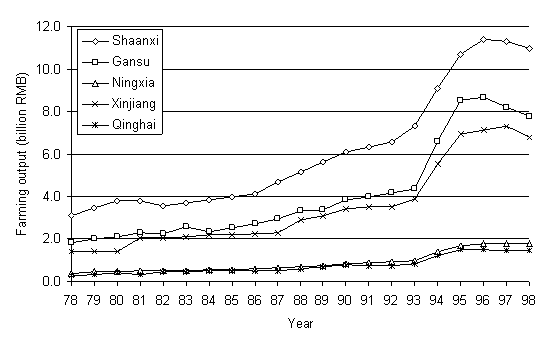
Figure 2. Time series plots of farming production in constant price for each provincial districts in northwestern China, during 1978 through 1998.

(Agricultural Systems, Volume 84, Issue 2, May 2005, Pages 155-169

Indexed by SCI,SSCI,

Impact factors of this journal
2003: 1.041 *
* Copyright ISI Journal Citation Report)